Contents
CBSE Notes for Class 7 Computer in Action – Charts in Microsoft Excel 2013
Charts are graphical representation of worksheet data. Data when represented in the form of charts makes it easier for users to quickly understand, compare and find patterns and relationships.
Whenever we have data based on numbers such as marks of students in different subjects, average temperature of various cities and so on, we prefer to represent it using charts. Data represented using charts can be easily understood, interpreted and analysed.
Excel provides various types of charts. It also provides options for customising and enhancing the presentation of a chart. Let us get started to learn more about charts in Microsoft Excel 2013.


ELEMENTS OF A CHART
Before we learn about creating charts, you need to have an understanding of various elements that make up a chart. A chart is described using various elements. Figure 3.3b displays the various elements of a chart.


Let us discuss these elements in detail.
- Data series: It refers to the set of worksheet data that are plotted in a chart (Fig. 3.3a).
- Chart title: It is the heading of a chart. It helps a user understand what the chart represents.
- Legend: The legend identifies each data series in a chart. Each data series is assigned a unique colour or pattern to differentiate one data series from another. It is usually displayed on one of the sides of the chart.
- Plot area: The plot area is the area containing the chart, axes and gridlines. In Figure 3.3b, the area inside the box is the plot area.
- Chart area: The chart area is the entire area containing the chart and all its elements—plot area, titles, legend and data table.
- Axes: The horizontal and the vertical lines that surround the plot area are called the axes. They are used as reference points for measuring the data values being plotted on the chart. The y-axis is usually the vertical line and contains value or data. The x-axis is usually the horizontal line and contains categories.
- Axes titles: These are the headings given to the x-axis and the y-axis. The titles help us in understanding what is being depicted on the axes.
- Gridlines: These are the horizontal or the vertical lines in the plot area. These lines make it easier to identify the value of each data point on the chart.
- Data marker: The data marker is any symbol such as a bar, an area, a dot or a slice used to represent a value in a chart.
- Data label: It is the title given to the data markers in a chart.
- Data table: It is the table containing the values for each data series usually displayed below the chart.
TYPES OF CHARTS
Excel supports various types of charts. The following are some of the different types of charts based on the worksheet data given alongside (Fig. 3.4).

Column Chart
A column chart is used to depict comparisons among different items of data or changes in data trend over a period of time. In this type of chart, values are represented on the vertical axis whereas categories are represented on the horizontal axis. Each bar in the chart represents value of one item of data. For example, the worksheet data shown in Figure 3.4 when represented in the form of a column chart appears as shown in Figure 3.5.

Bar Chart
A bar chart displays the comparisons among individual items as sets of horizontal bars. A bar chart is similar to a column chart except that in this type of chart, the values are represented on the horizontal axis whereas categories are represented on the vertical axis. For example, the worksheet data shown in Figure 3.4 when represented in the form of a bar chart appears as shown in Figure 3.6.

Pie Chart
A pie chart is used to plot only one data series. It is a diagram in the shape of a circle, divided into triangular sections that represent percentages of different quantities that add up to 100%. This type of chart is particularly useful when you want to show the relationship of individual items to the sum of all items in the series. For example, the pie chart depicted in Figure 3.7 displays the percentage of sales of different cars in the month of January.

Dougknut Chart
A doughnut chart is similar to the pie chart except that it can be used to plot more than one data series. Data series is represented by individual rings. Each section on a ring displays the contribution of an individual item to the total of all items in a particular series. For example, the doughnut chart depicted in Figure 3.8 represents the sales of cars in the month of January in the inner ring, February in the middle ring and March in the outer ring.

Line Chart
A line chart uses connecting dots to show trends in data over a period of time. Each line in the chart shows the changes in the value of one item. For example, to check the trend in the sales of cars month-wise, we can plot the worksheet data depicted in Figure 3.4 as a line chart (Fig. 3.9).

CREATING A CHART
The basic steps for creating a chart are the same no matter what type of chart you choose. Let us create a chart using the worksheet data given in the Figure 3.4.
Step 1
Select the range of cells containing the data (including the column titles and the row labels) to be plotted on the chart. For example, in the given worksheet (Fig. 3.10a), select cells A2:D6.

Step 2
Click on the insert tab
Step 3
Click and select the desired chart category in the Charts group. We will plot a Column Chart for the data series in this example. Click on the Column option in the Charts group. A drop-down list of chart subtypes is displayed.
Step 4
Select the desired chart sub-type. In this case, click on the Clustered Column chart sub-type. The chart appears in the worksheet. Two new tabs, Design and Format, appear in the Ribbon whenever you click on the chart (Fig. 3.10b). These tabs contain options for editing and formatting the chart.
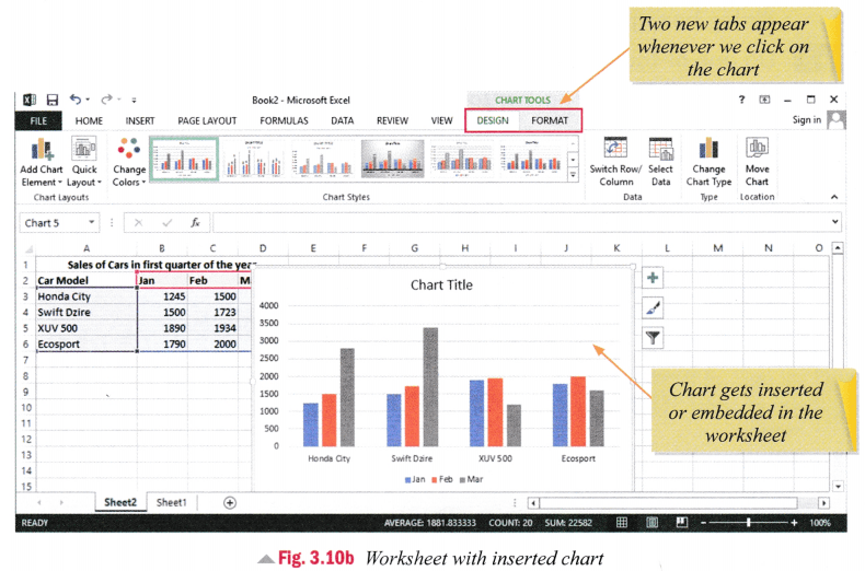
Placement of the Chart
By default, the chart is inserted or embedded in the worksheet. We can click on the chart and drag it to place it at any other position in the worksheet. We can also place the chart on another worksheet or a new sheet called the Chart Sheet.
Click on the chart and follow these steps to move the chart to a different sheet.
Step 1
Click on the Design tab (Fig. 3.11a).
Step 2
Click on the Move Chart option in the location group.The Move Chart dialog box appears (Fig. 3.11b).
Step 3
Do one of the following.
Choose New sheet option to place the sheet on a new chart sheet.
OR
Choose the Object in option and select the Sheet in which the chart should be placed as an object.
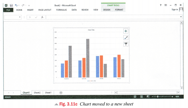
Step 4
Click on the OK button.
The chart moves to the new sheet (Fig. 3.11c).


ADDING CHART ELEMENTS
We can add various elements such as axis titles, chart title, data labels, data table and legend to enhance the readability of the chart. Click on the chart and use the Add Chart Element command present under the Design tab

Let us learn how to add elements.
Adding Axis Titles
To add axis titles follow the given steps.
Step 1
Click on the Axis Titles option in the Add Chart Element drop-down list (Fig. 3.13a).
Step 2
Do any of the following.
To add a title to a primary horizontal (category) axis, click Primary Horizontal Axis Title.
OR
To add a title to a primary vertical (value) axis, click Primary Vertical Axis Title.
An Axis Title box appears.
Step 3
Type the text in the Axis Title box or in the Formula bar. After typing the title, click outside the chart Fig. 3.13b.


Adding Ckart Title
To add chart title follow the given steps.
Step 1
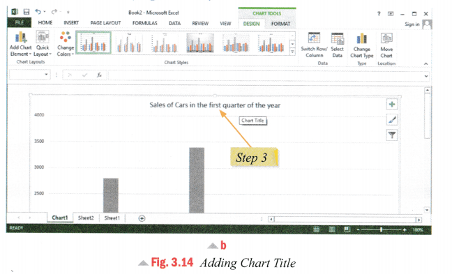
Click on the Chart Title option in the Add Chart Element drop-down list (Fig. 3.14a).

Step 2
Click on the Above Chart or Centered Overlay option. A Chart Title text box appears.
Step 3
Type the text in the Chart Title text box. After typing the title, click outside the chart (Fig. 3.14b).
Adding Data Labels
To add data label follow the given steps.
Step 1
Click on the Data Labels option in the Add Chart Element drop-down list

Step 2
Choose the appropriate option for the placement of labels.
Adding Data Table
To add data table follow the given steps.
Step 1
Click on the Data Table option in the Add Chart Element drop-down list (Fig. 3.16).

Step 2
Choose the appropriate option for the placement of data table.
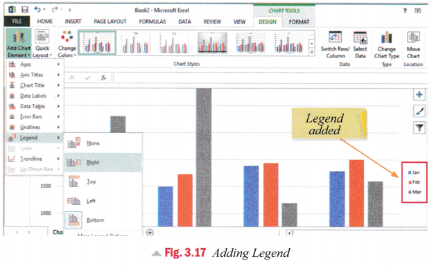
Adding Legend
To add legend follow the given steps.
Step 1
Click on the Legend option in the Add Chart Element drop-down list (Fig 3.17)
Changing the Chart Style
We can change the visual style of the chart any time after we have added the chart. Click on the chart and choose an appropriate style in the Chart Styles group on the Design tab (Fig. 3.18).

Words to Know
Chart: The graphical representation of worksheet data.
Axes: The horizontal and vertical lines that surround the plot area used as reference points for measuring the data values being plotted on the chart.
Chart area: The entire area containing the chart and all its elements such as plot area, titles, legend and data table.
Data marker: Any symbol such as a bar, an area, a dot or a slice that is used to represent a value in a chart.
Data series: The set of data values that are plotted in a chart.
Gridlines: The horizontal or vertical lines in the plot area of a chart.
Legend: A box that helps in identifying various plotted data series by assigning a unique colour or pattern to a particular data series in a chart.
Plot area: The area containing the chart, axes and gridlines of a chart.