With new discoveries and innovations constantly being made, the study of Physics Topics remains a vibrant and exciting field of research.
How will you prove that the surface of a charged conductor is an equipotential surface? and What is the Potential Resides Inside A Hollow Charge Conducting Sphere?
Definition: A surface containing points at the same potential in an electric field is called an equipotential surface.
Equipotential surfaces due to an isolated point Charge: In Fig., a few equipotential surfaces due to an iso-lated positive point charge have been shown. We know that, for

an isolated point charge q at a point O in vacuum, potential at a distance r is \(\frac{1}{4 \pi \epsilon_0} \frac{q}{r}\)[in SI]. So if a hollow sphere of radius r is drawn taking O as the centre, the outer surface of the sphere will be an equipotential surface, because potential at all points on the surface is equal to \(\frac{1}{4 \pi \epsilon_0} \frac{q}{r}\). The outer surfaces of all con-centric spheres so drawn will be equipotential surfaces. With O as centre, larger the radius of the sphere drawn, smaller will be the surface potential.
Equipotential surfaces due to a uniform electric field: A uniform electric field is represented by parallel and equi-spaced field lines. Equipotential surfaces in such a field would be normal to these field lines at every point in the field. Hence, each of these equipotential surfaces A, B, C would be plane and parallel to each other [Fig.]. The surfaces correspond to different potentials V1, V2, V3 respectively; but the potential at every point on any particular surface is the same.

In a strong electric field, the potential changes quickly along the direction of the field lines; in a weaker field, this change is slower. As a result, the spacing between successive equipotential surfaces, for a given fixed potential difference, is less for a stronger field [Fig. (a)] than that for a weaker field [Fig. (b)],

Equipotential surfaces for a pair of point charges:
In this case, the shape of the equipotential surfaces depends on the algebraic sum, at any point in the electric field, of the potentials generated by the two point charges separately. The equipotential surfaces
1. for two like charges of the same magnitude and
2. for two unlike charges of the same magnitude, have been shown in Fig.(a) and Fig.(b) respectively. In the figures, the blue and red lines represent the equipotential surface and field lines, respectively.

Properties of equipotential surfaces:
i) No work has to be done to move a charge from one point to another on an equipotential surface.
Work done to move a unit positive charge from one point to another is equal to the potential difference between the two points. Since potential at all points on an equipotential surface is equal, hence to move a charge from one point to another on an equipotential surface, no work has to be done.
ii) Field lines intersect the equipotential surface perpendicularly.
Let us consider two points A and B very close to each other on an equipotential surface S [Fig.].

Let the electric field intensity \(\vec{E}\), in the region AB , make an angle θ with the equipotential surface. Since A and B are very close to each other, AB may be taken as a straight line. Component of electric intensity E along AB = Ecos θ.
So work done to move a unit positive charge from A to B = Ecosθ × AB
From the property of an equipotential surface, we know that no work is done in moving a charge from one point to another on an equipotential surface.
∴ Ecos θ × AB = 0 or, cos θ = 0 [∵ AB ≠ 0 ; E ≠ 0 ]
or, θ = \(\frac{\pi}{2}\)
So the direction of field intensity is perpendicular to the equipotential surface. We know that the direction of electric field intensity and that of a field line through any point is the same. So it may be said that the field lines intersect equipotential surfaces normally.
By calculus: Let us consider two points A and B very close to each other on surface S [Fig.]. VA and VB are the electric potentials at the points A and B respectively. So, the potential difference between A and B is
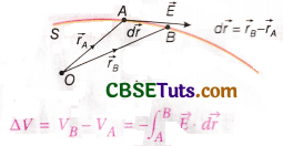
By definition, on an equipotential surface, ΔV = 0 i.e., \(\vec{E} \cdot d \vec{r}\)
So, \(\vec{E}\) is normal to d\(\vec{r}\). The latter being tangential to the curve, \(\vec{E}\) is normal to the surface represented by the curve.
iii) If there be a difference of potential between two different points of the surface of a conductor, charges will begin to flow from one point to the other until the potential becomes the same at the two points. So the surface of a charged conductor is an equipotential surface and charges on such a surfacer remain at rest.
iv) No two equipotential surfaces intersect each other. Any intersection would mean that the point of intersection corresponds to two different potentials; also, there are two electric field intensities at that point in two normal directions. These are impractical.
The surface of a charged conductor is an equipotential surface—experimental demonstration: We have already come to know that charge of a conductor resides on its surface. The surface charge density of a charged conductor depends on the shape of the conductor and is maximum at the region where its curvature is greatest. But the potential at every point on the surface of a charged conductor is the same and is quite independent of the shape of the conductor.
To verify it experimentally, an insulated pear-shaped conductor A is charged positively [Fig.]. The disc of an uncharged gold leaf electroscope is connected by a wire to a proof-plane. The electroscope is placed at such a large distance from the conductor that no electrical induction takes place in it.

The proof-plane is held by its insulating handle and brought in contact with the pear-shaped conductor. The proof-plane is moved to different parts of the surface and it is found that the divergence of leaves remain constant. This proves that the potential on a charged conductor is uniform, i.e., the surface of a charged conductor is an equipotential surface.
Potential Inside A Hollow Conductor
Though no charge resides inside a hollow charged conductor, potential at any point on the inner surface is equal to that at the outer surface of the conductor. This can be proved by the
following experiment.

An insulated deep hollow metallic vessel C is charged positively and it is placed at a
sufficient distance from a gold leaf electroscope [Fig.]. A proof-plane P is connected by a wire to the disc of the electroscope and is dipped gradually inside the vessel. The leaves of the gold-leaf electroscope would diverge; this divergence would be maximum when the depth of the proof-plane becomes sufficiently larger than the dimensions of the top opening. This divergence would not increase any more if the proof-plane is dipped farther, or is moved sideways.
As the divergence of the leaves indicates the magnitude of potential, it can be said that the potential inside the vessel is constant.
Now if the proof-plane is made to touch the outer surface of the vessel, the magnitude of divergence of the leaves does not change. This proves that the potential inside a charged hollow conductor is uniform, having the same value as that on its surface.
The potential inside a charged hollow conductor, V = constant. Hence, the electric field intensity,
E = –\(\frac{d V}{d x}\) = 0
This means that the interior of a hollow conductor is associated with no electric field and no field line.
E = 0 in a region corresponds to V=constant; it does not necessarily mean that V = 0 in that region.
Numerical Examples
Example 1.
Charge Q is distributed between two concentric hollow spheres placed in vacuum in such a way that their surface densities of charge are equal. If the radii of the two spheres be r and R (R> r), calculate the poten-tial at their centre.
Solution:
Let the charge on the smaller and the bigger spheres be Q1 and Q2, respectively.
∴ Q = Q1 + Q2
As the surface densities of charge of the two spheres are equal,

Example 2.
Charges +2 × 10⁻⁷C, -4 × 10⁻⁷C and +8 × 10⁻⁷C are placed at the vertices of an equilateral triangle of side 10 cm in air. Determine the electrical potential energy of this system of charges.
Solution:
Distance between any two of the charges, r = 10 cm = 0.1 m.
The electrical potential energy of the system of charges is the algebraic sum of the potential energies of each pair of the charges. For air, permitivity is ε0.
Potential energy of the system of charges

The negative sign indicates that 0.0216 J work is to be done to transfer the charges from their positions to infinity.
Example 3.
In vacuum, three small spheres are placed on the circumference of a circle of radius r in such a way that an equilateral triangle is formed. If q be the charge on each sphere, determine the intensity of electric field and potential at the centre of the circle.
Solution:
Let O be the centre of the circle [Fig.]. Three spheres are placed at the points A, B and C on the circumference of the circle. ABC is an equilateral triangle.

Resolving the above intensities along A O and perpendicular to AO we have,
intensity along AO = EA – EB cos 60° – ECcos60°
= \(\frac{1}{4 \pi \epsilon_0}\left[\frac{q}{r^2}-\frac{q}{r^2} \times \frac{1}{2}-\frac{q}{r^2} \times \frac{1}{2}\right]\) = 0
intensity perpendicular to AO
= EA cos 90° + EB sin 60° – EC sin 60°
= \(\frac{1}{4 \pi \epsilon_0}\left[0+\frac{q}{r^2} \sin 60^{\circ}-\frac{q}{r^2} \sin 60^{\circ}\right]\) = 0
∴ Resultant intensity at O = 0
and electric potential at O = \(\frac{1}{4 \pi \epsilon_0}\left[\frac{q}{r}+\frac{q}{r}+\frac{q}{r}\right]\) = \(\frac{3 q}{4 \pi \epsilon_0 r}\) units
Example 4.
A charged particle q Is thrown with a velocity v towards another charged particle Q at rest. It approaches Q up to a closest distance r and then returns. If q Is thrown with a velocity, what should be the closest distance of approach? [AIEEE ‘04]
Solution:
Let the closest distance of approach be r’.
From the principle of conservation of energy we have,
kinetic energy = electrostatic potential energy.
In the first case,
\(\frac{1}{2} m v^2\) = \(\frac{1}{4 \pi \epsilon_0} \cdot \frac{q Q}{r}\) …. (1)
In the second case,
\(\frac{1}{2} m(2 v)^2\) = \(\frac{1}{4 \pi \epsilon_0} \cdot \frac{q Q}{r^{\prime}}\) …. (2)
Dividing equation (1) by equation (2) we get,
\(\frac{1}{4}\) = \(\frac{r^{\prime}}{r}\) or, r’ = \(\frac{r}{4}\)
Example 5.
In vacuum, four charges each equal to q are placed at each of the four vertices of a square. Find the intensity and potential of the electric field at the point of inter section of the two diagonals. [HS ‘07]
Solution:
Let the length of each side of the square be a. Accord-ing to the Fig.,
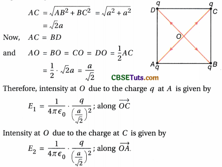
These two intensities being equal and opposite balance each other.
Similarly, intensities at O due to the charges at B and D being equal and opposite balance each other. So the intensity at the point of intersection of the two diagonals is zero.

Example 6.
Three point charges q, 2q and 8q are to be placed on a 0.09 m long straight line. Find the positions of the charges so that the potential energy of this system becomes minimum. In this situation, find the intensity at the position of the charge q due to the other two charges?
Solution:
Let the charge 2q be placed in between the charges q and 8q and the distance between q and 2q be x metre [Fig.].
So, the distance between 2q and 8q = (0.09 – x) m

∴ Potential energy of the system,

So, the charge 2q is to be placed at a distance of 0.0235 m, i.e., 2.35 cm from the charge q.
Electric field intensity at the position of the charge q due to the other charges,
E = 9 × 10⁹ × \(\frac{2 q}{x^2}\) + 9 × 10⁹ × \(\frac{8 q}{(0.09)^2}\)
= 9 × 109 × 2q\(\left[\frac{1}{(0.0235)^2}+\frac{4}{(0.09)^2}\right]\)
= 4.148 × 10¹³ q N ᐧ C-1